Langton’s Ant

Moved to new blog

Langton’s Ant is a turmite governed by simple rules whose outcome is both unpredictable and intresting. The path taken by the ant generates some surprising shapes, never appearing when you would expect them to, but a seemingly random moments. This article describes the rules behind Langton’s Ant, shows some of the images formed and provides a Python programme to simulate the ant.

Langton’s Ant

Chris Langton is a biologist, and the founder of the field of artificial life. One of his simplest and most intresting creations is Langton’s Ant. It is quite important theoretically, but it also has some intresting practical applications.

The ant’s world consists of a grid, possibly infinite, but limited in our example:

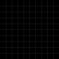
The ant always moves through this grid one step at a time. It’s direction and it’s effect on the grid is defined by 3 simple rules:

1. If the ant is on a black square, it turns right 90 degrees.
2. If the ant is on a white square, it turns left 90 degrees.
3. When the ant leaves a square, it inverts colour.

It is fairly obvious that the ant’s movement will leave a coloured trail. When asked, most people would guess that either no patterns show or that some basic symmetric images appear. What actually happens is this.

For the first 50 or so steps, it just seems to move around randomly, and then at step 52, you get a heart:

For the next 300 or so steps, the ant seems to draw random shapes, ofter erasing what it had drawn before. At about step 383 you get something that looks like this:

Next you get what’s technically known as a mess. The ant’s movement degenerates into chaos. No more patterns are observed:

By now, you are probably thinking: “Well yes. Simple rules, so at first you get simple patterns, but as the board gets more and more complex, the simple rules can’t handle it, so the ant moves randomly”. Well that’s right, up until about step 10000; that is when you start getting highways.

The highways the ant draws are intresting shapes. You can see one at the bottom of the next image. It is the diagonal bit going down and right. To build then, the ant seems to move in circles, the last row forcing it to draw the next. Thus, the ant continues to draw until something gets in its way. In this simulation, because the screen wraps around, the ant eventually gets back to the mess, where it starts moving randomly again.

What’s intresting is that, after some time, the ant starts building highways again. Actually, there is no known way to stop it. The only hindrance here is that the board is finite so it has a tendency to fill up. Anyway, here’s what the board looks like at step 97049:

The Programme

The following is a simple programme written in Python and using PyGame.

The variables that control the display and the board are at the top of the programme. They are heavily commented so there shouldn’t be any problems.

Here’s the code in Python (langton.py):

#************************************************
# Rules of the game
#	1. If the ant is on a black square, it turns
#		right 90 and moves forward one unit
#	2. If the ant is on a white square, it turns
# 		left 90 and moves forward one unit
#	3. When the ant leaves a square, it inverts
#		colour
#
# SEE: http://mathworld.wolfram.com/LangtonsAnt.html
#************************************************

import sys, pygame
from pygame.locals import *
import time

dirs = (
		(-1, 0),
		(0, 1),
		(1, 0),
		(0, -1)
		)

cellSize = 12 # size in pixels of the board (4 pixels are used to draw the grid)
numCells = 64 # length of the side of the board
background = 0, 0, 0 # background colour; black here
foreground = 23, 23, 23 # foreground colour; the grid's colour; dark gray here
textcol = 177, 177, 177 # the colour of the step display in the upper left of the screen
antwalk = 44, 88, 44 # the ant's trail; greenish here
antant = 222, 44, 44 # the ant's colour; red here
fps = 1.0 / 40 # time between steps; 1.0 / 40 means 40 steps per second

def main():
	pygame.init()

	size = width, height = numCells * cellSize, numCells * cellSize

	pygame.display.set_caption("Langton's Ant")

	screen = pygame.display.set_mode(size) # Screen is now an object representing the window in which we paint
	screen.fill(background)
	pygame.display.flip() # IMPORTANT: No changes are displayed until this function gets called

	for i in xrange(1, numCells):
		pygame.draw.line(screen, foreground, (i * cellSize, 1), (i * cellSize, numCells * cellSize), 2)
		pygame.draw.line(screen, foreground, (1, i * cellSize), (numCells * cellSize, i * cellSize), 2)
	pygame.display.flip() # IMPORTANT: No changes are displayed until this function gets called

	font = pygame.font.Font(None, 36)

	antx, anty = numCells / 2, numCells / 2
	antdir = 0
	board = [[False] * numCells for e in xrange(numCells)]

	step = 1
	pause = False
	while True:
		for event in pygame.event.get():
				if event.type == QUIT:
					return
				elif event.type == KEYUP:
					if event.key == 32: # If space pressed, pause or unpause
						pause = not pause
					elif event.key == 115:
						pygame.image.save(screen, "Step%d.tga" % (step))

		if pause:
			time.sleep(fps)
			continue

		text = font.render("%d " % (step), True, textcol, background)
		screen.blit(text, (10, 10))

		if board[antx][anty]:
			board[antx][anty] = False # See rule 3
			screen.fill(background, pygame.Rect(antx * cellSize + 1, anty * cellSize + 1, cellSize - 2, cellSize - 2))
			antdir = (antdir + 1) % 4 # See rule 1
		else:
			board[antx][anty] = True # See rule 3
			screen.fill(antwalk, pygame.Rect(antx * cellSize + 1, anty * cellSize + 1, cellSize - 2, cellSize - 2))
			antdir = (antdir + 3) % 4 # See rule 2

		antx = (antx + dirs[antdir][0]) % numCells
		anty = (anty + dirs[antdir][1]) % numCells

		# The current square (i.e. the ant) is painted a different colour
		screen.fill(antant, pygame.Rect(antx * cellSize + 1, anty * cellSize + 1, cellSize -2, cellSize -2))

		pygame.display.flip() # IMPORTANT: No changes are displayed until this function gets called

		step += 1
		time.sleep(fps)

if __name__ == "__main__":
	main()

It is intresting to note that although you know all the rules that govern the ant's universe, you cannot predict its movement without resorting to simulation. This just goes to show that knowing the rules of the components at the lowest level might not help you understand the system as a whole.

That’s it. Have fun with the code. Always open to comments.

 

Speeding up Dijkstra’s Algorithm 1

Moved to new blog

In this article, I describe a simple (adds less than 1min of work) way to speed up Dijkstra’s Algorithm for finding the single source shortest path to every node in a graph.

In a previous post I described the simple O(n²) implementation of the algorithm. Here, I focus on a method that will probably speed up the algorithm.

Why Bother

The previous implementation of the algorithm ran in O(n²) time, where n is the number of nodes in the graph. This means that for a graph of, say 100 nodes, it would do about 100 * 100 = 100000 calculations. Considering that computers nowadays are said to be able to do about 100000000 (a hundred million) calculations per second, we’re fine, and the programme will finish in well under a second. But what if we have a graph with 100000 nodes? This might take 100 seconds to run. Now we’re in trouble. We need a faster algorithm.

The two most common ways to speed up Dijkstra’s Algorithm are to implement the finding of the closest node not yet visited as priority queues. Usually heaps or Fibonacci Heaps are used for this purpose (Fibonacci Heaps were actually invented for this).

Heaps are somewhat difficult to implement and Fibonacci Heaps are horror to implement. Incidentally, there’s a very easy of speeding it up.

Just Use Queues

The idea is to simply use queues instead of priority queues. This way provides nowhere near the same level of speedup (the algorithm is still O(n²)), but it makes it run faster, on average, by a factor of 4.

Some bad news: a carefully crafted graph could slow this algorithm down to O(n³). As a rule, graphs in real life are never like this, and, as the method isn’t widely known, test sets for contests are not written to catch this optimisation.

Now for the good news: it’s shockingly easy to write. Compare the old dijkstra1() with the new dijkstra2().

void dijkstra1(int s) {
	int i, k, mini;
	int visited[GRAPHSIZE];

	for (i = 1; i <= n; ++i) {
		d1[i] = INFINITY;
		visited[i] = 0; /* the i-th element has not yet been visited */
	}

	d1[s] = 0;

	for (k = 1; k <= n; ++k) {
		mini = -1;
		for (i = 1; i <= n; ++i)
			if (!visited[i] && ((mini == -1) || (d1[i] < d1[mini])))
				mini = i;

		visited[mini] = 1;

		for (i = 1; i <= n; ++i)
			if (dist[mini][i])
				if (d1[mini] + dist[mini][i] < d1[i]) 
					d1[i] = d1[mini] + dist[mini][i];
	}
}

void dijkstra2(int s) {
	int queue[GRAPHSIZE];
	char inQueue[GRAPHSIZE];
	int begq = 0,
	    endq = 0;
	int i, mini;
	int visited[GRAPHSIZE];

	for (i = 1; i <= n; ++i) {
		d2[i] = INFINITY;
		visited[i] = 0; /* the i-th element has not yet been visited */
		inQueue[i] = 0;
	}

	d2[s] = 0;
	queue[endq] = s;
	endq = (endq + 1) % GRAPHSIZE;


	while (begq != endq) {
		mini = queue[begq];
		begq = (begq + 1) % GRAPHSIZE;
		inQueue[mini] = 0;

		visited[mini] = 1;

		for (i = 1; i <= n; ++i)
			if (dist[mini][i])
				if (d2[mini] + dist[mini][i] < d2[i]) { 
					d2[i] = d2[mini] + dist[mini][i];
					if (!inQueue[i]) {
						queue[endq] = i;
						endq = (endq + 1) % GRAPHSIZE;
						inQueue[i] = 1;
					}
				}
	}
}

What’s changed? First, we define several new variables. These, together, make up the queue:

int queue[GRAPHSIZE];
char inQueue[GRAPHSIZE];
int begq = 0,
    endq = 0;

Next, during the initialisation part of the function, we mark all nodes as not being in the queue.

for (i = 1; i <= n; ++i) {
	/* OTHER INITIALISATIONS (look at the programme) */
	inQueue[i] = 0;
}

Now, add the source node to the queue.

queue[endq] = s;
endq = (endq + 1) % GRAPHSIZE;

What does this do? The first line add s to the end of the queue. The second line moves the end of the queue one step to the right (I’ll explain a few paragraphs down). The modulo operation here is not really necessary, but I like to be consistent.

At this point we’ll start looping. When do we stop? The idea here is that a node is in the queue when its neighbours need to be updated (i.e. when a new shortest path might be found leading to them). So, we stop when the queue is empty. Note that this occurs when begq == endq and not when !(begq < endq). So, while (begq < endq) is incorrect because, in one case, begq will be greater then endq.

What was the first thing we did in the loop? We were supposed to find the closest node not yet visited. Now, we merely take the first node from the queue.

mini = queue[begq];
begq = (begq + 1) % GRAPHSIZE;
inQueue[mini] = 0;

Here, the first element is pop’d out of the queue, the head of the queue is moved one step to the right and the element is marked as not being in the queue. The problem with queues in general, and this one in particular is that the part of them that actually hold the elements tends to move around. Here, every insert moves the tail one step to the right and every pop moves the head one step to the right. Consider the following sequence of operations:

Moves 1 through 8 clearly show that, while the size of the information content of the queue changes erratically, it constantly moves to the right. What happened at 9? The queue got to the end of available memory and wrapped around to the beginning. This is the purpose of (begq + 1) % GRAPHSIZE and (endq + 1) % GRAPHSIZE. It turns 7, 8, 9, etc. into 1, 2, 3, etc. But won’t endq overrun begq? No, the use of inQueue guarantees that no element will be inserted in the queue more than once. And as the queue is of size GRAPHSIZE, no overrun is possible.

So far, so good. One last modification: when we update the distance to a node, we add it to the queue (if it’s not already in it).

for (i = 1; i <= n; ++i)
	if (dist[mini][i])
		if (d2[mini] + dist[mini][i] < d2[i]) { 
			d2[i] = d2[mini] + dist[mini][i];
			if (!inQueue[i]) {
				queue[endq] = i;
				endq = (endq + 1) % GRAPHSIZE;
				inQueue[i] = 1;
			}
		}

Comparing the speed

When I first wrote this, I wanted to be able to check that it outputs correct results and I wanted to see how much faster it is. The following programme does both. The function cmpd() checks the output against that given by the simple implementation and the various clock() calls littered through the code time the two functions.

Here’s the code in C (dijkstra2.c):
Note: Source might be mangled by WordPress, consider downloading the file.

#include <stdio.h>
#include <time.h>

#define GRAPHSIZE 2048
#define INFINITY GRAPHSIZE*GRAPHSIZE
#define MAX(a, b) ((a > b) ? (a) : (b))

int e; /* The number of nonzero edges in the graph */
int n; /* The number of nodes in the graph */
long dist[GRAPHSIZE][GRAPHSIZE]; /* dist[i][j] is the distance between node i and j; or 0 if there is no direct connection */
long d1[GRAPHSIZE], d2[GRAPHSIZE]; /* d[i] is the length of the shortest path between the source (s) and node i */

void dijkstra1(int s) {
	int i, k, mini;
	int visited[GRAPHSIZE];

	for (i = 1; i <= n; ++i) {
		d1[i] = INFINITY;
		visited[i] = 0; /* the i-th element has not yet been visited */
	}

	d1[s] = 0;

	for (k = 1; k <= n; ++k) {
		mini = -1;
		for (i = 1; i <= n; ++i)
			if (!visited[i] && ((mini == -1) || (d1[i] < d1[mini])))
				mini = i;

		visited[mini] = 1;

		for (i = 1; i <= n; ++i)
			if (dist[mini][i])
				if (d1[mini] + dist[mini][i] < d1[i]) 
					d1[i] = d1[mini] + dist[mini][i];
	}
}

void dijkstra2(int s) {
	int queue[GRAPHSIZE];
	char inQueue[GRAPHSIZE];
	int begq = 0,
	    endq = 0;
	int i, mini;
	int visited[GRAPHSIZE];

	for (i = 1; i <= n; ++i) {
		d2[i] = INFINITY;
		visited[i] = 0; /* the i-th element has not yet been visited */
		inQueue[i] = 0;
	}

	d2[s] = 0;
	queue[endq] = s;
	endq = (endq + 1) % GRAPHSIZE;


	while (begq != endq) {
		mini = queue[begq];
		begq = (begq + 1) % GRAPHSIZE;
		inQueue[mini] = 0;

		visited[mini] = 1;

		for (i = 1; i <= n; ++i)
			if (dist[mini][i])
				if (d2[mini] + dist[mini][i] < d2[i]) { 
					d2[i] = d2[mini] + dist[mini][i];
					if (!inQueue[i]) {
						queue[endq] = i;
						endq = (endq + 1) % GRAPHSIZE;
						inQueue[i] = 1;
					}
				}
	}
}

int cmpd() {
	int i;

	for (i = 0; i < n; ++i)
		if (d1[i] != d2[i])
			return 0;

	return 1;
}

int main(int argc, char *argv[]) {
	int i, j;
	int u, v, w;
	long t1 = 0,
	     t2 = 0;

	FILE *fin = fopen("dist2.txt", "r");
	fscanf(fin, "%d", &e);
	for (i = 0; i < e; ++i)
		for (j = 0; j < e; ++j)
			dist[i][j] = 0;
	n = -1;
	for (i = 0; i < e; ++i) {
		fscanf(fin, "%d%d%d", &u, &v, &w);
		dist[u][v] = w;
		n = MAX(u, MAX(v, n));
	}
	fclose(fin);

	for (i = 1; i <= n; ++i) {
		long aux = clock();
		dijkstra1(i);
		t1 += clock() - aux;
		aux = clock();
		dijkstra2(i);
		t2 += clock() - aux;
		if (i % 10 == 0) {
			printf("%d / %d\n", i, n);
			fflush(stdout);
		}
		if (!cmpd()) {
			printf("\nResults for %d do NOT match\n", i);
			break;
		}
	}
	printf("\n");

	printf("Dijkstra O(N^2):\t\t%ld\n", t1);
	printf("Dijkstra unstable:\t\t%ld\n", t2);
	printf("Ratio:\t\t\t\t%.2f\n", (float)t1/t2);

	/* printD(); */

	return 0;
}

And here’s a big 1200 node graph: dist2.txt.

Have fun and good luck. Always open to comments.